Grain growth
References
Introduction
Grain growth is a microstructure evolution phenomenon that occurs in polycrystalline materials after solidification. Some grains are growing at the cost of shrinking other grains or crystallites of a specific orientation. Consequently, the average grain size increases, accompanied by reducing the number of grains in the material.
The driving force for grain growth is the curvature-driven grain boundaries between different crystallites with different orientations. The energy of these grain boundaries adds excess free energy to the system. Therefore the grain boundary energy is the driving force for the movement of the grain boundaries, and the system evolves towards minimizing the total free energy.
As a result, the material's microstructure proceeds to reduce the entire area of the interfaces. The kinetics of grain boundaries influence the interfacial migration, the energy and mobility of these boundaries control how the grain structure evolves [1].
Simulation setup
OpenPhase® has a built-in example, "NormalGG", to show you the simulation of grain growth. The driving force is curvature driven, which is the only contribution to the transformation.
The example shows a normal grain growth with isotropic interface energy and mobility, and the user can modify the example to account for the anisotropy of both contributions.
The microstructure generation is obtained using the Voronoi tessellation from points (the centre of grains) randomly distributed in the box. The user can change the starting number of grains directly in the example file.
The "ProjectInput.opi" contains all the input parameters related to the simulation. The user can vary the file upon his particular use. The simulation conditions for the specified example has been modified in the "ProjectInput.opi" and considered as:
| Parameter | Symbol | Value | Units |
|---|---|---|---|
| Grid Size | - | 4003 | Cells |
| Number of Grains | - | 18000 | - |
| Grid spacing | Δx | 1 x 10 -7 | m |
| Time steps | Δt | 1 x 10 -1 | s |
| Interface width | η | 6Δx | m |
| Grain boundary energy | σ | 1.0 | Jm-2 |
| Grain boundary mobility | μ | 1 x 10 -14 | m4(Js)-1 |
| Boundary conditions | PBCs | Periodic | - |
Results
Microstructure evolution
Fig. 1 (right) shows the evolved microstructure at 900 [s] for isotropic grain boundary energy and mobility with around 4000 grains. The simulations show that the system exhibits normal grain growth. It is noticeable in Fig. 1 that the isotropic grain boundary energy does not have any effect on the overall evolution of the microstructures (see pole figure). The distribution of our plane normal does not change with time and has no effect on the simulation, and this is clear because we have both isotropic grain boundary energy and mobility.
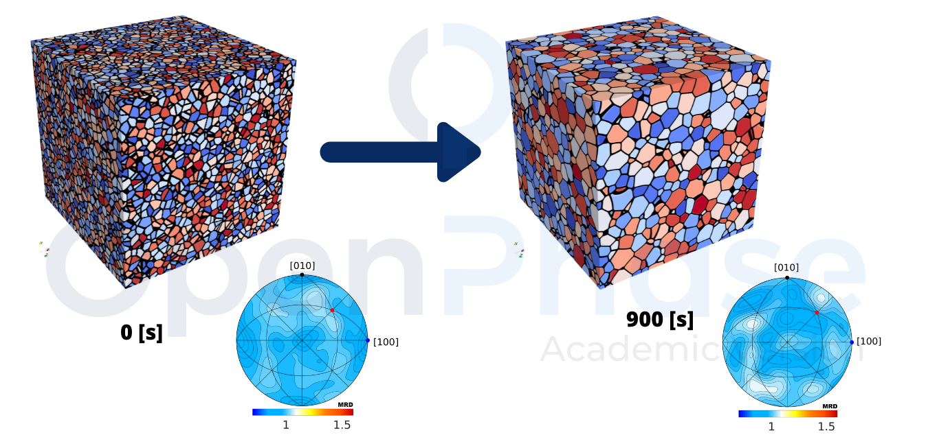
Figure 1: Microstructure of the simulated grain growth.
Average grain size
The evolution of the grain size distribution during grain growth is shown in Fig. 2 compared with Hillret 3D theory [2]. The x-axis in the plot displays the relative grain size with respect to the critical grain size [3]. The system soon evolves from its original restricted distribution to a larger one. After a few timesteps, the simulation's grain size distribution closely resembles Hillert's prediction and remains almost constant for a long time. The number of grains that exist reduces, though. Nonetheless, the peak of the grain size distribution gradually shifts to the left at a later stage. The frequency of large grains on the right-hand side of the distribution increases at the same time, and the distribution becomes more symmetric around "1". While the pace of change in the grain size distribution is slowing, the symmetric grain size distribution maintains its shape for a reasonably long time, as shown in the graph below. These results are in line with the work by Kamachali et al. [4] and Kim [5].
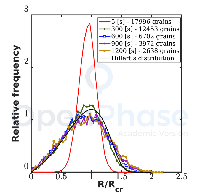
Figure 2: Grain size distribution.
Related Topics